Anything For A Map - Part 0

10 Dec 2016

On The Heels of The Pioneer Corps

Mapping the footprints of the men who faced the thicket, built drifts across rivers, played the debut soccer and rugby matches in a country.

Background

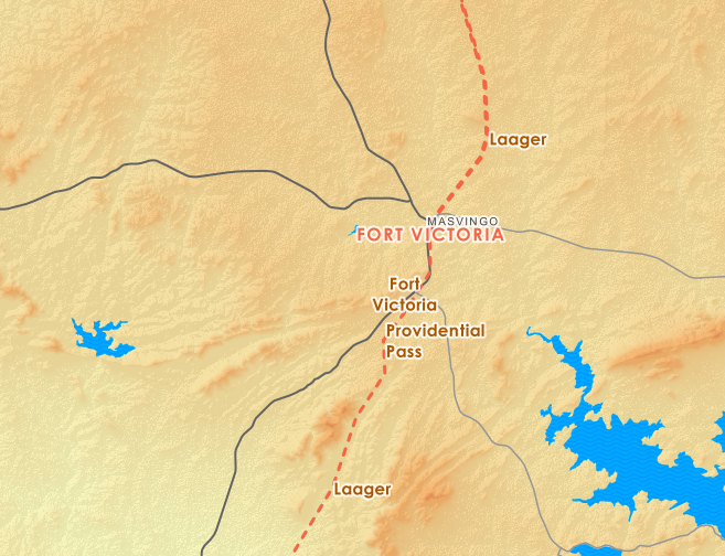
I am enthused by maps and more so good cartography. I will scrounge any document just to map the two or more places mentioned there. Perchance while working with an old topomap of Zimbabwe, I bumped into small crosses that represented features of historic significance. Of special intrigue were locations identified as Fort and Laager (pictured above). As I Google-dug some more on these, I came across an article, Pioneer Forts in Rhodesia 1890-1897. My interest grew as I read a gripping account by Horste.(The Historic Publication) He chronicles how in 1890, the Pioneer Column’s escort of British South Africa Company’s Police progressed into present day Zimbabwe. I had read and heard about this in my history classes, that was then, I am all maps now!

BUSY ?:~ Cut To The Chase.***

Why?

• Well, I’m am oft looking for something to map (and the narrative by Hoste is too good to waste!)
• To have a ‘cartographic-perspective’ of how the historic route impacted the development of existing roads and towns.
• Get a ‘feel’ of the topography the column faced.
• Tinkering!

Get There Fast

1. Vector Data Preparation

2. Raster Data Preparation

3. Map Creation

4. Map Serving

5. Challenges/ Observations

6. Results

My conception of the map was a route, points and relief map that stood out, with a subtle backdrop of existing roads and features. I had bumped into carto works with tilemill, in particular Toner. I had to ‘broad-read’ on various carto projects. For starters, I had an undated, georeferenced 1:250 000 topography map of Zimbabwe(Rhodesia). I opened a blank QGIS project, which had the following CRS settings. This was the basis of other work to follow:

1. Vector Data Preparation

Key Points

• (route_points.shp): The first task was to create spatial data for key points. Sources of information was the topo map and the narrative by horste. Editing in QGIS is pretty straight forward. This route_points.shp shapefile would contain three fields: name, type, notes, arrival. These fields I came up with after several passes of the narrative. Name would be used to label the point, type to style (in Tilemill) , notes for additional information on the point and arrival to capture the date the Pioneer Corps arrived at the ‘point’.

Route Plotting

• (route_track.shp): Route plotting logic was to join the points with a line. To refine the route, I took a hint from the narrative - avoid the hills and follow watersheds.

Route Buffer

• (route_50km_buffer.shp): Within QGIS Processing Toolbar, the next operation was to buffer an area around the route. I would use this extent to map the route and generally clip other data for the project. I decided on a buffer radius of 50km. A guy named Selous had ‘pre-scanned’ the road ahead and gave indication as to where the column should march through. Additionally, I intended to use terrain data with 30m spatial resolution and 50km would give me ~1700 pixels on either side of the route. This should provide good ‘terrain-context’.

2. Raster Data Preparation

I am a fan of relief maps. I could just spend hours just panning a good representation of terrain so this stage would give me great pleasure! For this section I intended to follow these tutorials - Working with terrain data and Using TileMill’s raster-colorizer. I however ended up emulating this in QGIS. Which gave excellent results!

Relief Map

• QGIS handles raster data easily. I was going to use the SRTM Version 3, 30m DEM data set. The project area (route_50km_buffer.shp) was covered by 14 elevation data tiles. In QGIS I merged the tiles to form one dem tif. [Toolbar] – Raster – Miscellaneous – Merge, to come up with (route_dem_raw.tif)

• I clipped the merged elevation model with (route_50km_buffer.shp), this resulted in a ‘along-route’ tif viz (route_dem_50km_buf.tif).

• In line with this tutorial, I was to create a hillshade first. My machine is setup with OSGeo4W so running gdal commands was supposed to be a breeze. so I ran

  gdaldem hillshade -co compress=lzw route_dem_50km_buf.tif route_dem_hillshade.tif
  

• A relief map was next. Firstly I styled (route_dem_50km_buf.tif) in QGIS: 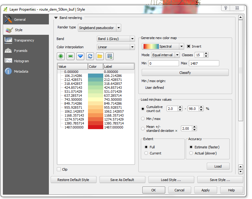. It turned out the 15 equal interval classes and a spectral colour map gave an unsatisfactory relief map. Pleasantly, QGIS permits the export and import of colour ramps. So I got busy editing the 15 interval ramp I had generated - a painstaking task, but I prevailed. So with the colour_ramp.txt, which I had also checked in QGIS, I ran

  gdaldem color-relief route_dem_50km_buf.tif colour_ramp.txt route_dem_colour_relief.tif
  

• Next up was slope shading which is a two way procedure. First

  gdaldem slope route_dem_50km_buf.tif route_dem_slope.tif
  

• Then secondly, the actual slope shade

  gdaldem route_dem_colour_relief.tif -co compress=lzw route_dem_slope.tif slope-ramp.txt route_dem_slopeshade.tif
  

  As explained here, make sure to use the slope.txt file so that the “color-relief command can use it to display white where there is a slope of 0° (i.e. flat) and display black where there is a 90° cliff (with angles in-between being various shades of grey).”

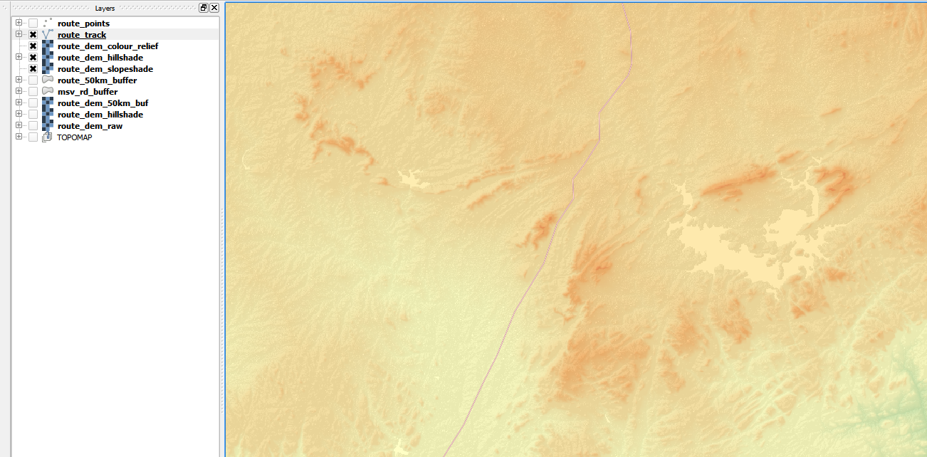
Just for fun, I loaded the three elevation data files (tifs) created above into QGIS and styled them with the transparencies indicated in the Tilemill tutorial, viz colour_relief: 10% transparent, hillshade: 60%,slopeshade: 40%. The result was astounding!

3. Map Creation

Osm Toner

To provide cartographic contrast and temporal context I wanted a subtle background and osm toner seemed the best choice. The procedure is outlined succinctly here.

• First , I got a subset of OpenStreetMap data relevant to my project from BBBike.org from which one can clip data to custom boundaries. (Aside: I only discovered this site while hacking this project, indeed giyf! )

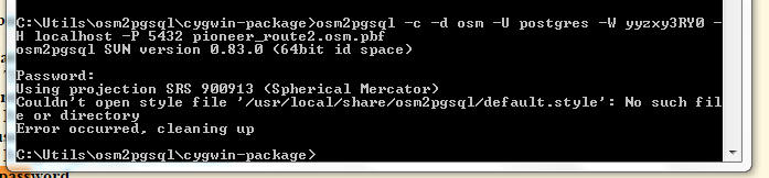
• Next was loading the OSM data into a PostGIS database. I already had a Postgres Installation. So in PgAdmin III, I created a database and named it osm. After that the actual loading of the data had to be done. More information on running osm2pgsql can be found here. For this I downloaded cygwin-package.zip and extracted to a folder. After saving my custom OSM data (pioneer_route2.osm.pbf) to the same folder as osm2pgsql.exe. 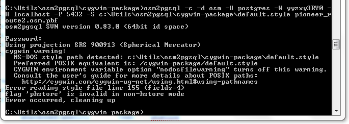I ran the command and got error: After some Googling and amends, another error After this, I had to download default.style from the web. Re-running the command again, now with the style available…another error: , I tried to address that with some Postgis chops. 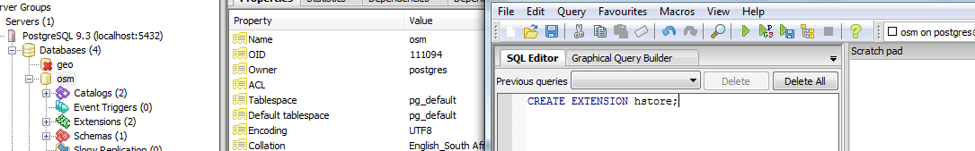. That also did not give solace. I opened the file in Notepad++ and commented out line 155 to 160 of default.style in the text editor. I figured this wasn’t that important for my intended use - map styling. .

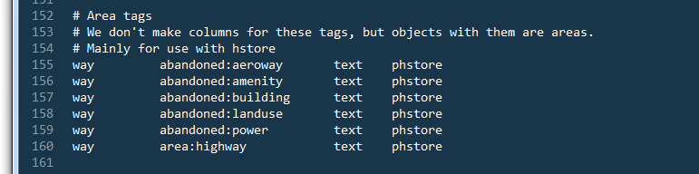  Tilemill

• Running config.py : In accordance with the tutorial, I edited the python file accordingly and successfully ran make.py. My project was automatically created. Unfortunately several things went wrong with this setup - among them, having to download a ~300MB file (I have access to very limited bandwidth).

• Since I had some exposure to Tilemill, I had an idea of how stuff was structured so decided to take the ‘brute-force’ route to having a Toner-Template setup. I resorted to modifying the DC-Streets project (which is auto-setup with an installation of TileMill):

  • I prepared my custom osm data (previously loaded into PostGRES ) to match that on the DC-Streets project. The (shapefile) schema had to be exact - viz field for field so that styling and labelling would be smooth.

  • Now what remained was to tweak the major CartoCSS colour styles using gray scales only. For this I simply edited the highway.mss and used ColorBrewer to more accurately pick greys that would represent the roads and color-hex to decode the ‘hashed’ alpha-numeric characters.

More Styling in Tilemill

• Creating the terrain map

  • Using the raster layers I had prepared in QGIS in Stage 2. above, I loaded them in TileMill and styled them as I had in QGIS. Amazeballs! This would serve as the base layer for the other data except at higher zoom levels viz > 13. (I concluded the relief display range from playing with the visualisation in TileMill).

• Adding detail - The Route and Stop Points

  • Adding the Column route was straight forward as I had styling in highway.mss to emulate.

  • With the Stop points I had a little reading of the manual (aka Google) to do as the *open-streets-dc templates did not include any points styled. I wanted some fancy symbolisation. Through trial and error I got satisfactory results eventually for the various zoom levels.

  • Rivers and streams were essentially lines and polygons and I had the template as a starting point.

• Labelling

  • My Intention was emphasise history and ‘background’ the present. So I made my labels for the column landmarks coloured. Luckily the place names in open-streets-dc were already black and white. So I didn’t have to touch those.

  • A serious challenge was to avoid label conflicts and also at the same time display landmarks and labels at the same time. Again reference to the manual saved the day. Used text-dx: and text-dy: extensively in the CartoCSS.

Exporting The Mapwork

This stage was the most exciting for me - who doesn’t want to see the fruit of their labour?! TileMill gives you a preview of what the export will be like in the WYSIWYG manner so there’s no crossing of fingers to what the output will be like, just a demand for patience as the export runs.

After two unsuccessfully runs I had to explicitly define the RCS for all the layers in my project.(those were set to Auto-Detect). I defined my export parameters - MBTiles, Bounds, Centre - saw the software estimated 8 hours to completion of the run. Luckily it was night so I went for some shut-eye.

Come morning there was my 237MB MBTiles file!

I fired up QGIS to take a look. I recalled QGIS supported these. The result was not so impressive - had a grainy feel to it. TileMill had rendered it smoothly so I knew it was not my data. I remembered a Portable MBTiles viewer. I couldn’t quite recall the name to I consulted my GitHub account (anything I think might be of interest to me I put on the Watch list ) - there it was TileStream Portable.

I loaded my MBTiles per instruction and my pannable map ….

So one can actually give a friend, client a pannable map on a USB Stick loaded with the MBTiles being served by the TileStream Portable. (*I’ve read on the inter-web companied serving imagery as MBTiles *)

4. Map Serving

*I will not go into detail describing step-by-step this part of my exercise as it detracts from the intention of this blog post. Summary will only be given since with Stage 3 above, the Mapping exercise would be complete.

How-to serve the resultant map was largely inspired by the following blog post which I emulated closely - Setting up a Cloud MBTiles Server with Benchmarks (You can also find the screencast in my Github Repo).

Leaflet was used as the Mapping Client. I had had a historic stint with The Bootleaf Template and I started there - with a clone of that repository. I spend considerable time in SublimeText 3 editing the template to suit my needs.

5. Challenges/ Observations

Some points to note in the representation of wok done here:

• I had to deal with data of varying spatial scales - Topo map, Elevation data, Openstreetmap data, etc.

• For some stretch of the route between explicitly mentioned stop points, the narrative by horste was not sufficient to accurately approximate the route the pioneer corps took.

• There is error inherent in the the use of Laagers plotted from the topo map since no temporal information was given. These could well have been apart historically.

• Laagers are a temporary feature hence their representation must be interpreted as being virtual, temporally obsolete from point to point. (The corps were moving forward and ‘broke laager’ as they progressed!)

• Notice that after Fort Victoria, the track becomes dual. According to Horste “We now made two parallel roads, about fifty yards apart, as it had been decided to have a double line of wagons, instead of the long cumbersome single line that we had had up to then.”

• Gave water bodies prominence (represented in colour) - little might have changed since 1890 just as is the case with terrain. Not withstanding the construction of dams since then.

6. Results

I have served all the data relating to this project to a GitHub repository.

You can link directly to the resultant map here - The Pioneer Column Map

#postscript

• I traversed many ‘technology domains’ in this exercise and it was fun. That has helped me know a comfortable bit of everything. Linux Server administration! Database Server Management - remember my PostGIS instance?
• After my experience with TileMill on this project, I decided to move to (Mapbox) Studio. No need to remain in ‘legacy mode’ - I am a geohipster!
• TileMill may be ‘old’ and out of active development but it does pack a punch! Additionally you don’t have to ‘connect’ to MapBox to use it like its successors - MapBox Studio and MapBox Studio Classic.

Commits, Pathways and Cogs

12 Nov 2016

Of Commits and Cogs

The Cloud: For A Rainy Day Reason

So, when I came to an abode hit by a ‘forced entry’, my heart sank. Not only was my trusty HP 450 - i3 15.6 Notebook missing but the pending ‘commits’ to my github file and blog repository. Oh, the GeoHipster sticker, and only one, on the lappy was gone too. A week later I got a 1GB RAM Machine donation from a friend. Without giving it a thought, my way back up was via Portable QGIS for spatial data work. With fingers crossed, I should be able to set up my blogging environment again (Aha! I had documented the procedure as a blog post).

From this unfortunate encounter i learnt that

• The cloud is there for a reason. Stay in the cloud to avoid a rainy day.

• Commit often. It’s a great backup.

The loss of my machine was a major drawback to the blogging commitment I had made. In it all though, It dawned on me from a friend’s loss that

You can steal a man’s resource or equipment but they’ll always have the idea and dream with them.

So I continued to blog, albeit offline.

The takeaway from this post is: Commit Often, Backup Often, Avoid the umbrella.

Drive The Cogs

Recently, well 2015-2016, I got to sit in on a number of meetings at my day job. I enjoyed the conversations, dialogue rather but, it all got me thinking. My greatest contribution was to do with spatial, after the fact, at the back of my mind I would be thinking how can all this we are discussing about be made into some cool system?

People around the table were mostly planners, higher management decision makers. Technical details is not on their lips but, technical gets my endorphins going. Technical, systems, database …

I’m forced to take out the magnifying glass and inspect the path I am treading. The short of it: I enjoy pushing and seeing the cogs turn!

Anything for a Map - Part 1

04 Sep 2015

On The Heels of The Pioneer Corps

Mapping the footprints of the men who faced the thicket, built drifts across rivers, played the debut soccer and rugby matches in a country.

Background

So, as I was working on some project and the corresponding write-up for a blog post, I got a ‘technology’ interruption. The key data for the project was ready now and the other processing was still ongoing TileMill, GDAL, ASTER.. what not.

CartoDB was the interruption and particularly Odyssey.js. My (initial) intention was to make a pannable map with an ‘old’ theme. Since this was going to be a spatio-temporal kind of a map I decided to give Odyssey.js a go.

Tire-kicking

So in one afternoon I had a reasonable visualisation going! Having a CartoDB account was one of the requirements for this exercise and I had long back signed up for a free account when CartoDB came on to the scene. I went with the Torque Template on Odyssey.js. The point data I uploaded to my CartoDB account, simply added a ‘integer’ field to represent time. It wasn’t difficult to figure out how the story could be put together using Markdown. And after two hours or so….voila!

The Map Story

#postscript

• The experience I had with Markdown helped me to quickly compile my story.
• I used a great tool by Ben Balter to upload a document of the narrative I used to plot the points in the visualisation to my GitHub account via the browser!
• Apart from the expediency with which one can make a animated visualisation of one ’s data, there’s somewhat a restriction on the cartography front. Thus I will still continue with my initial intention on creating an old map.
• Take away from all this is that there are great tools out there to help one do great things with minimal effort.

Cartoportation

08 Jul 2015

Map-Teleportation

In a matter of minutes I was ‘cartoported’ from 2015 to circa 1980. It all started when I turned the Google Maps Navigator on. In a matter of 10 minutes I was totally disoriented as to where I was going. This was exacerbated by the season of the year. Sunset quickly turned to night. I only wished it was summer time where sunset can be experienced at 20:15 and not 17:58. The sacrifice I had made for some costly mobile data was about to count for nothing.

The first mistake was over-reliance on the battery life of a Samsung Galaxy S4 Mini. At 35% you’d think you still have some hours of ‘play-time’ with the gadget. Two hours maybe, but that’s before you turn on GPS with ‘Locating method’ set to highest. Add to the mix a bumper-to-bumper traffic jam, and the ETA starts to increase, the distance falling at a snail’s pace.

I am one for no fiddling with a gadget while driving (#itcanwait), so I ignored the thing and enjoyed the diversity of cars passing left and right. The battery low warming was drowned by the engine sounds all around. Even if I had heard it, it didn’t matter because I had no in-car charger.

Stop and Look

5km or less after off-ramping from the busy national road into an arterial road, the phone went dead. Disorientation quickly set in. The comfort of just listening to “in 500 m take the left exit” was gone. I tried to remember; What was that road again that I was supposed to branch to? Was I to turn right or left after the third street? I quickly realised I didn’t remember and the information boards were only confirming what I already knew and not the finer detail I sought - when am I supposed to make that left?

As it turned dark, I stopped at a Caltex fuel/ service station. After strolling the place a bit, I found the favour of a petrol attendant whom a later entrusted with my trusty Galaxy. Ten minutes was the most I was gonna allow myself to remain ‘deaf’. I had already accumulated considerable time since my battery had died.

Cartography By Hand 101

The 10 minutes recharge (with the wrong charger) got me 15% of charge. I had pen and paper ready as I switched the phone on. I wrote down key contacts, turned on Location, ran the Maps app, searched my address and did my sketching. I think I did well. You be the judge…

I got my confidence back. Drove slower to as to glance at the sketch now and then.

In all this I learnt that one with a variety of tools in their toolbox is at an advantage.

#postscript

• You probably have looked at the ‘survival’, must-haves for your car but the pen and paper do come in handy. So does some Cartography skills.

The Thin Data Pipe

08 May 2015

I recollect a time, seven or so years back, I was at a place where I celebrated the successful download of a 10MB installation file. I would compress it (WinRar), chop it up and then save it to several 1.44MB diskettes!

We have progressed well since that time but I still find myself using a thin pipe to tape to the internet!

A Tinkeror’s Necessity

For any ‘Tinkeror’ internet access is an indespensable assay but, the average Joe has to tinker more to get ahead. With the boom and proliferation of FOSS tools, ability to download at will is largely a given, the means, quite the contrary - for my part of the world. The connections to the interweb are there and the speeds are reasonable. The challenge is what you trade for to get your data chunk. Some great geo-toys even assume you’re always connected to the internet. Well, thanks to initiatives like the Smart Cape, I can budget the 500MB data allocation per month to download only critical programs to my ‘workbench’ or trusty S4 Mini mobile phone. But wait, I need to

$ rake deploy

to have my latest blog post published, and that requires some data currency. Thanks to git, I don’t need to push a file horde, just a simple markdown text file and a few pics. The 150MB/ month I get from my Service Provider atomises within four days of receiving it - provided I decide to be conservative about visiting Facebook. Trouble starts when I need that 729MB Landsat 8 file to check out what is happening this rainy season with the once disastarous Tokwe-Mukorsi Dam.

I could download just the bands I need but, even that would deplete my monthly quota by (~59MB x 3) 35% for a true colour band combination. This is too much to sacrifice just for one project. Work arounds have to be fathomed, working with a D-Link 3G 21Mbps, USB Modem and Mobile phone (Mobile hotspot functionality).

# Wait For Night

I’m sure am not the only tinkeror who sacrifices sleep now and then.

Work all night, Sleep all day, Wake up at 8pm really confused

– @lyzidiamond

At night, one can get a bit of reasonably prized data. I ran a USSD request on my service provider (07 May 2015) and got ‘Night Express’, 1GB for R10. Remember this will be chowed by a single landsat scene multiband image and would cost me a few hours of snooze.

An alternative service provider has a similar data deal:

But there is a catch, I get to sleep a bit later. Yay!

# Sip or Chow & Work

There are 101 restaurants and Cafes with ‘Free-Wifi’ access. But having to trade 50MB/ day for your phone number and email address is a bit too much. Don’t even start on the idea of moving from Cafe to Cafe until a project is done. Sipping on a cup of coffe for two hours! Really?

Google Search is like a pencil and scrap pad. I transfer mental notes to there. More often than not I have typed Define:{Mind drift idea here} in that nifty search box. The thought that my browser is connected to the interweb never occurs in all of this.

# A Mesh Of All

Well, a 40Mbit/s ADSL line in the house, enabling one to read ‘Done!’ after a repository clone command simultaneously with the lifting of the finger off the ‘Enter’ key would be ideal. Until then, patience and data budgets remain the order of the day for the average Joe.