

Relations, I Mean, Tables Galore
03 Jul 2018SCT Part 2
Embracing Text
In the previous blog, we explored how we can load (explicitly) spatial data, initially in shapefile format, to a geopackage. In this post we explore the loading of relations a.k.a table to the geopackage. Again, data from the Open Data Portal is used.
Data Is Rarely Clean!
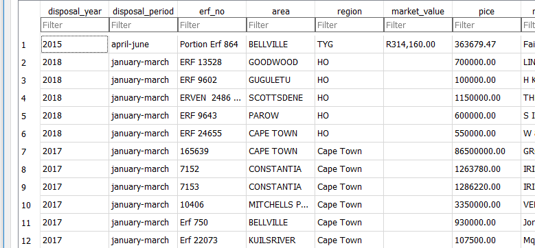
We will explore “Data showing City land that has been disposed of.” The data is spread over several spreadsheets covering various time periods. In some instance yearly quarters. The data custodian is given as “Manager: Property Development & Acquisitions city of capetown.”
In the data wrangling process using LibreOfficeCalc, the open source equivalent of MS Excel. Several attributes will be learnt about the data. Especially that which hinders a refined data structure. Issue will be varied, among them:
- Not all records being filled in.
- No consistency to period of registrations.
- Inconsistent formatting of currency.
- Sale price included or excluded VAT inconsistently.
- Typos in area names.
- A regions field which definition could not be got from the Open Data Portal.
To improve the data we may end up
- Adding some fields to improve schema
- Concluding area field = Suburb Name (per suburb_layer from previous blog post)
- Matching the area field names to match up with Suburb Name in the Base Suburbs reference data we adopted.This procedure inadvertently modifies data from it’s original structure. However, knowledge of local suburb boundaries and place locations means the impact will be minimised.
Casual inspection reveals
- A lot of sales to churches and trusts. Possible follow-up questions would be. Was this influenced by any legislation in a particular year? Which year saw the largest number of sales to churches?
Loading Tabular Data To Geopackage
With the Land Disposals data, covering several years, curated and consolidated into one spreadsheet. It is time to import this data into our geopackage. Here are the steps to do it:
1. From the Spreadsheet application (OpenOfficeCalc), Save file as and choose Text CSV (Comma Separated Values).
To load the Text File to the geopackage we use any one of the two approaches.
Method 1: Using QGIS
1. Start Q if not already running.
2. Select Add Delimited Text. This is a large comma icon with a (+)plus sign. When you load the file, it will likely look like the screenshot below. (Note that the image shown here is of a file that would have undergone considerable pre-processing. Especially on field names and data types in cells.)
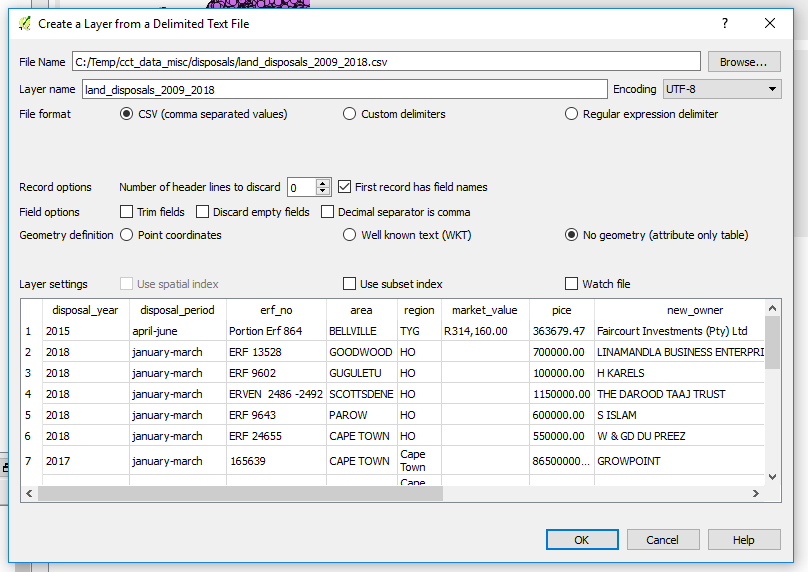
Make the selections as shown above. In particular ‘No Geometry’.
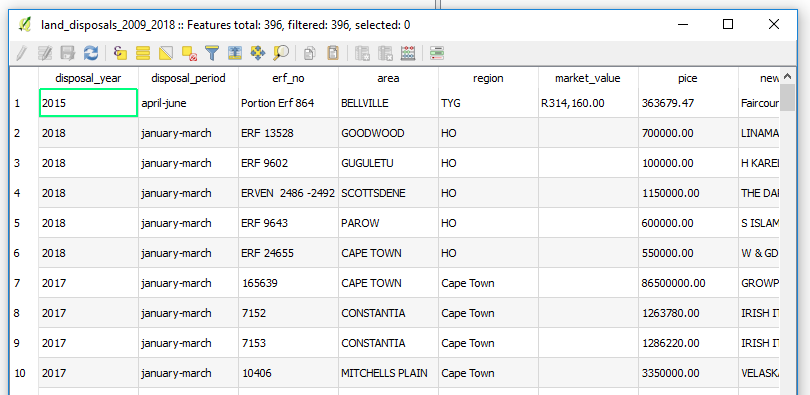
Opening the table in Q we see the data we just imported.
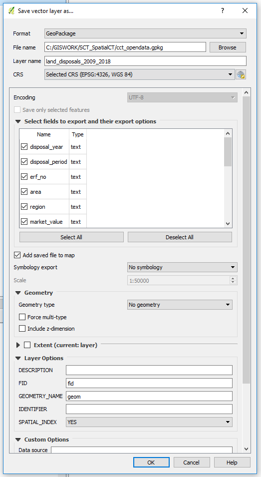
Now let’s save this to the GeoPackage.
3. Rick Click the Layer name, –> Save As. Then specify the location of the geopackage. In the dialog box that comes up, under Geometry, choose No Geometry. (We are just importing a non-spatial table.).
That’s it!
Let’s explore an alternative way of getting the text file into the GeoPackage.
Method 2: Using SQLite Browser
1. Open the GeoPackage in the SQLite Database Browser.
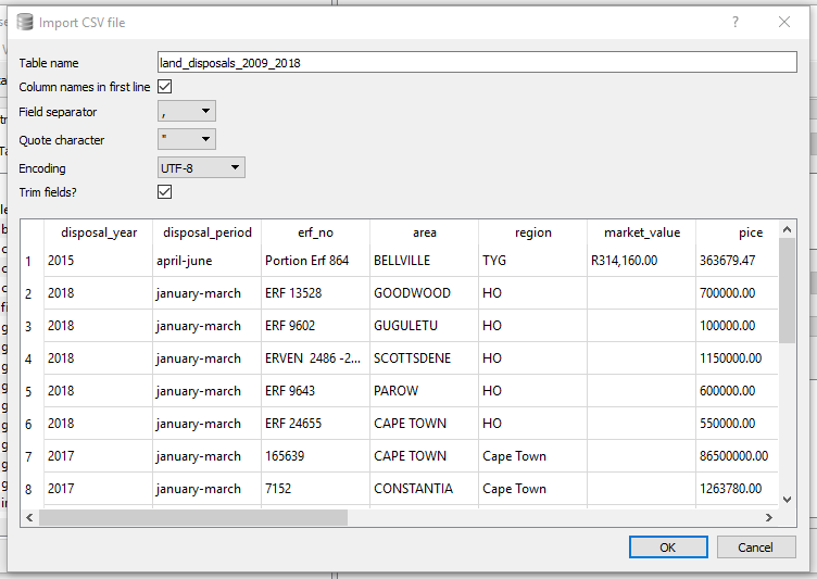
2. Do File –> Import –> Table from CSV. Check on; Column Names in first line and Trim fields?. Separator is comma.
Done!
3 Switch to the Browse Data tab to see what we have just loaded.
A Review: What To Choose
On inspecting the table loaded with QGIS and SQLite Browser. Somehow Q correctly and auto-magically distinguish text and numeric field data types. SQLite Browser made everything type “TEXT” in this particular case.
Let’s experiments some more with our data.
Close SQlite Browser and switch to QGIS. (It is good practice to close one application when accessing data from another. Particularly if you are to do editing.)
Launch DB Manager and Browse to the geopackage. Let’s see how many distinct suburbs do we have in this table. Start the SQL Windows and run…
SELECT DISTINCT  area FROM  land_disposals_2009_2018
ORDER by area ASC;
we get 102 records . We see there is NULL in first entry so we really have 101 records. On close inspection we notice there are a lot of typos in some names.
We will need to clean this data if we are to have meaningful analysis later on.
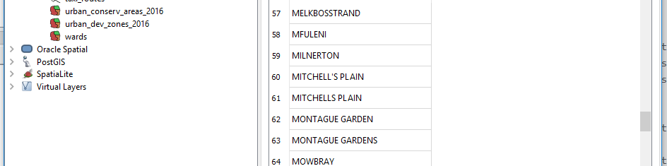
Let’s check the suburbs layer and see how the data compares
SELECT DISTINCT  NAME FROM  suburbs
ORDER by NAME ASC;
We get 773! This is gonna be interesting, especially getting exact matches.
Before cleaning the data further, lets see if we can ‘connect’ the suburbs and land_disposals datasets.
SELECT  * FROM suburbs
JOIN land_disposals_2009_2018
ON suburbs.NAME = land_disposals_2009_2018.area;
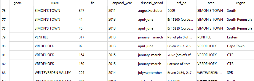
Yep! We have some hits.
We are going to be basing our analysis on the suburbs layer so we use that layer for a base and format subsequent datasets after that it as much as possible. Cleaning can be done in QGIS user interface editing or better still in the sqlite database (geopackage) using SQL.
#PostScript
The take away is that GeoPackage can store tables, no sweat.
The join operation used above is simplistic. One would need to appropriately use LEFT, RIGHT, INNER JOIN.
I used:
- QGIS 2.18 (DB Manager)
- DB Browser for SQLite 3.10.1
- SublimeText 3.1.1