

A Bright Square Kilometre
31 Dec 2018SCT Part 4
All That Glitters
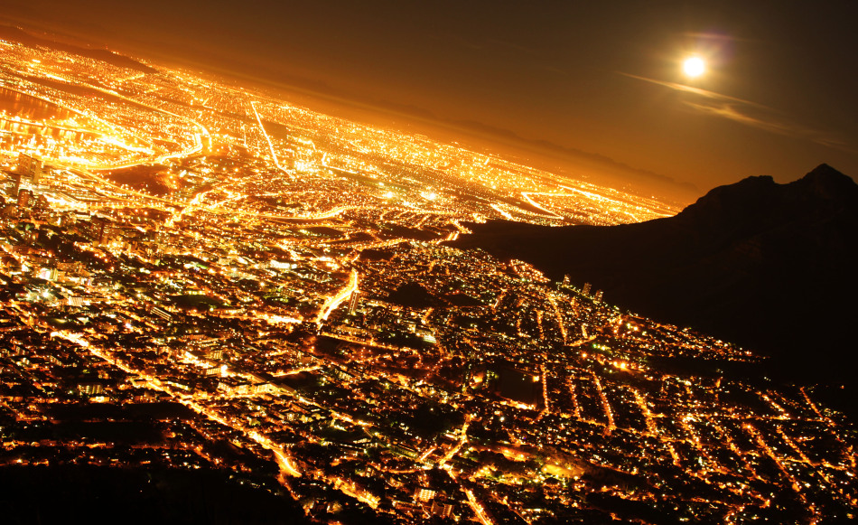
Image credit - Gathua’s Blog
The above is a typical representation of Cape Town night lighting. How would that look like from space? One way to answer that is demonstrated here but, the data used there is quite coarse. This post is on a similar approach with the further investigation of finding the brightest spot on a Cape Town night. Data on the location of street lights was used as provided on the Cape Town open data portal.
Some Assumptions
- Street lighting is the only lighting at night time at a place.
- All street lights are represented (no broken light).
- The dataset is complete and accurate (temporally).
- All the lights have identical lumens.
- [Other implied assumptions.]
Public Lighting
The subject data is described as “Location of street light poles and area lighting (high-masts) in the Cape Town metropolitan area.” - Public Lighting 2017.zip
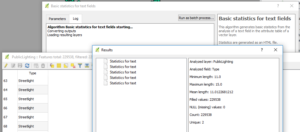
In Q, I ran Statistics for text field to find out how many unique lighting types there were. Just two - Streetlight and High-mast Light. A total of 229 538 lights.
The distinctiveness of street light types persuaded me to give greater weight to the High-mast Light. So, an additional assumption -
High-mast Lighting is twice as bright as just Streetlight lighting.
So in Q I created a weight field and populated it appropriately.
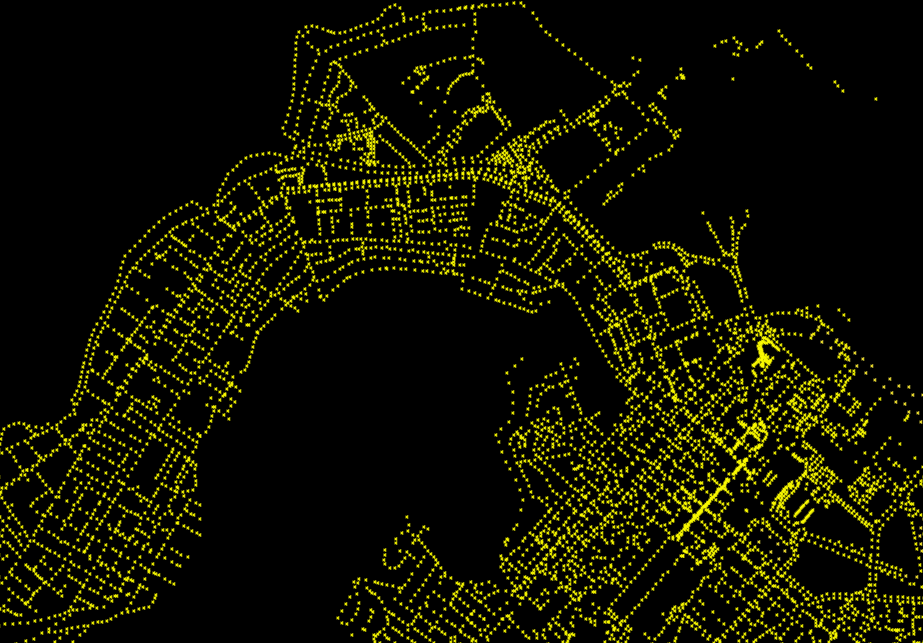
To scratch the curiosity itch. The lighting in Q, for the CBD and surrounds.
Boot Strapped Visualisation
If you haven’t heard of Kepler.gl you must check it out. I handles your geodata in the browser and does some amazing things.
First step is to convert the shapefile to csv, json or geojson. In Q this is achieved via right click on the layer and Save As.
Load the CapeTown_Public_Lighting.csv in Kepler.gl
(On loading the CapeTown_Public_Lighting.csv in Kepler.gl the weight field was being interpreted as type Boolean and not just Integer. It turns out this was a bug (December 2018). I quickly remembered this as I am actively ‘watching’ the Kepler.gl github repository)
As a workaround I used weights of 100 and 200 for the StreetLights and High-mast Light respectively.
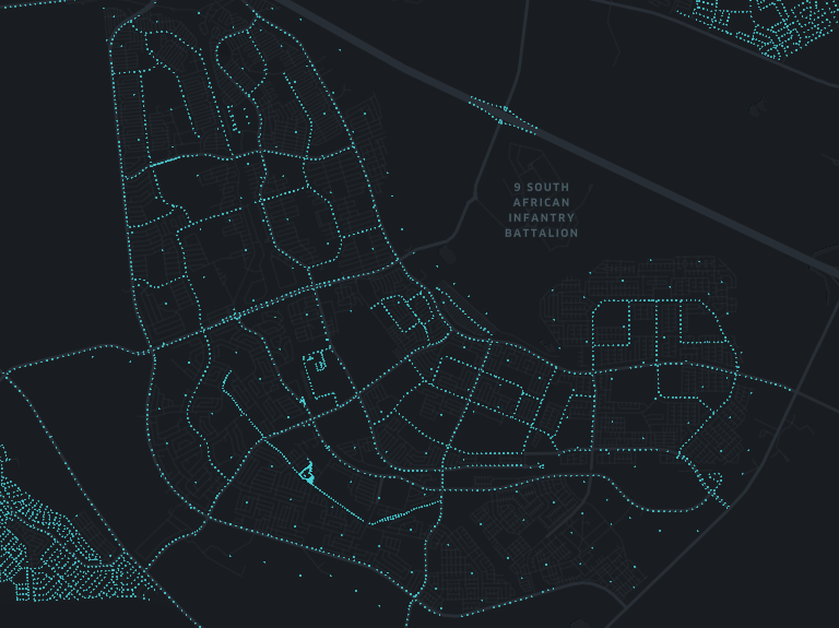
Panning around the map, the above caught my eye. Turns out the more isolated dots are high-mast lights. Actually in Kepler, you can filter/ view a type at a time or together using different colours and a whole other options.
Our objective of finding the brightest spot requires we aggregate the points data. That is home turf for Kepler. With a few clicks we have this;
We are looking for The Brightest Square Kilometre and we factor in the assumption high-mast light = 2 X Streetlight.
So in order to get to calculating the correct area for the hexagon being employed by Kepler, I got to asking.
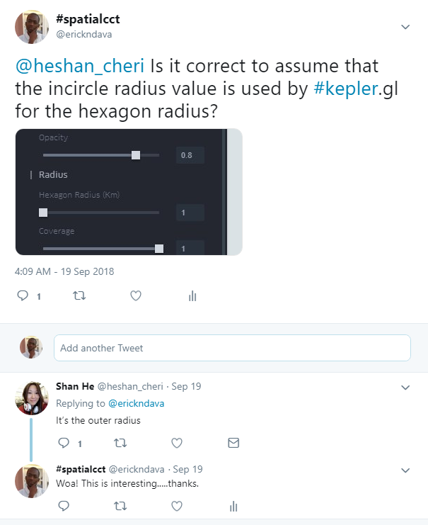
Taking a hint from here and using the formula
A = ½• n • r² • sin( (2π) / n)
where:
- A is the area of a polygon
- r is the outer radius
- n is the number of sides
I got the radius as 0.6204 km
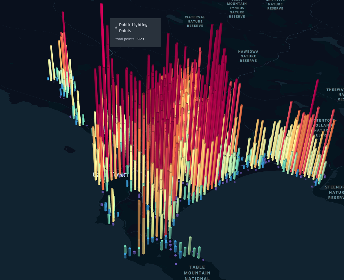
Under Radius Tab, Enter Radius value of 0.6204 and decrease the Coverage (base area of the hexagon being visualised) Switching ON The Enable Height Tab - Enter a reasonably high Elevation Scale, The HeighT is based on Point Count. High Precision Rendering turned ON.
These parameters aid quick identification of the ‘tallest’ hexagonal column hence the brightest square kilometre. With a count of 923.
Light Weight
To take into account the weight of the light type (high-mast vs street light), we add another data layer (a duplicate of the CapeTown_Public_Lighting.csv really), apply a weight filter Add a Layer based on this and style it with similar parameters to the first Layer. (At the time of writing this post, a filter when applied to a dataset affects all the layers based on it. Hence the need to duplicate the dataset with this approach.)
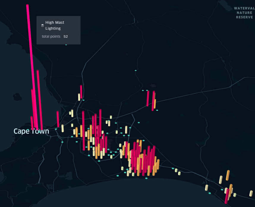
With a highest count of 52 per the square kilometre. Even doubling high mast lighting for impact falls short of the 871 (923 - 52) of ‘StreetLight’ alone.
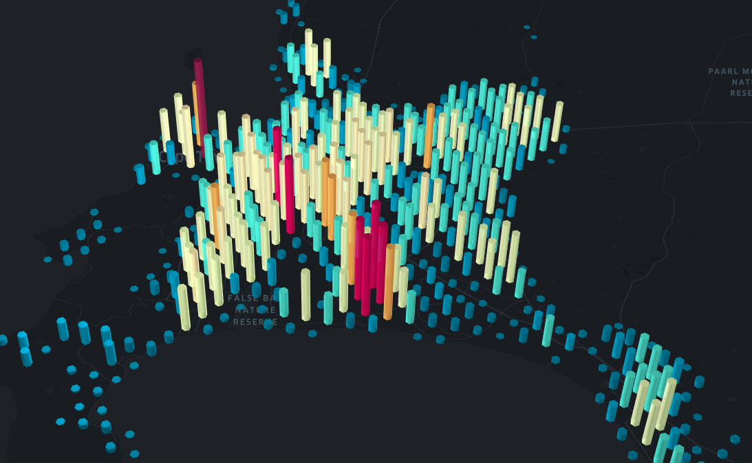
Now styling the High Mast Lighting with grey scale…so we can see the two together.
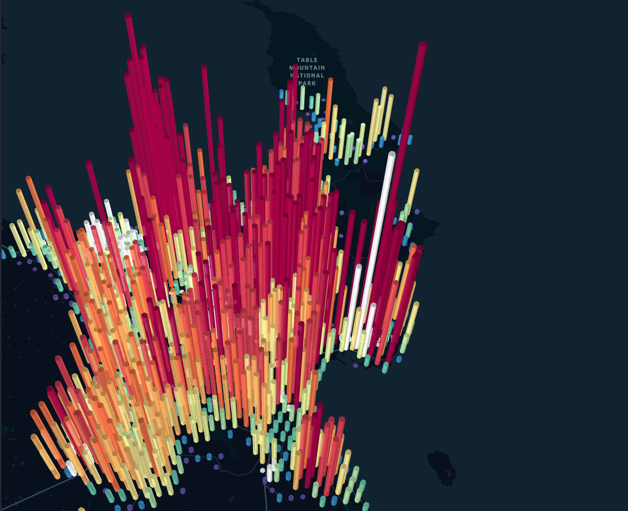
There is apparent correlation - Highly lit areas also have high mast lights. High Mast ~ ‘white’ columns.
You can interact with the Street Lights Map below.
#PostScript - Replicate
Kepler.gl is under active development and new features are being added continuously including some fascinating ones on the developers’ road map.
One of the features is the ability to share a visualisation easily. So here goes:
-
The Data and Settings ~ for this exercise can be downloaded here.
-
Download the file to your local drive and open it from The Kepler.gl Website.