2. The Data - Spatial

[A Data Science Doodle]

Defining Geography

One Area, Many Versions

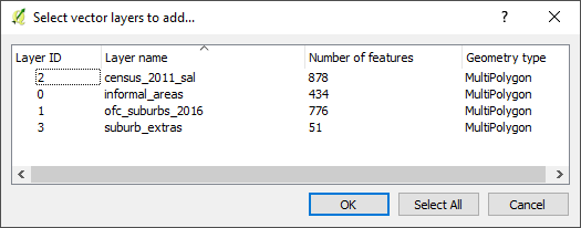
Inspection of the service request data led to the inference of the underlying place definition. Suburb(s) in this post will be used to refer to a place of geographic extent and not strictly per the make-up of a suburb.As main reference, the Official Planning Suburbs from here were adopted. Due to the shortcomings of the Official Planning Suburbs data (792 records), there was need to have many layers of reference for the bounds within which a service request falls.

The service request data also alludes to the usage of informal settlement names when defining the geography of a service request. Informal Area Data was sourced from here. Unfortunately the domain was decommissioned but, the metadata is here.

Another places data adopted was the Census 2011 Small Areas Layer downloaded from DataFirst, (data). This layer offers a finer grained place name demarcation the census Small Areas.This layer is useful in instances were population has to be factored in. Service requests are geolocated to a ‘smaller’ area which better approximates the original service request origin/ destination.

Therefore

Suburbs Data = Official Planning Suburbs + Census Small Area  + Informal Area + Any Other Reference Frame

The spatial data was loaded to a geopackage for further geo-processing.

A Good Frame

Getting Structured

The majority of the service requests were not geocoded or where geolocated to a suburb centroid and that called for a gazetteer of sorts. Inorder to have such a geographic frame the sourced data had to be collated and cleaned.

The exercise was dual:

(i) Trimming the unnecessary and some geoprocessing.

(ii) Ensuring spatial data integrity.

Part (i)

For the four layers (Official Planning Suburbs +Census Small Area + Informal Area + Extra suburbs) I did the following:

1. Created field name suburb and made the names upper-case.

2. Cleaned/ removed hyphens and other special characters from names.

3. Deleted spatial duplicates. In QGIS, ran “Delete duplicate geometries” from Processing Toolbox.

4. Found and deleted slivers in polygons data.

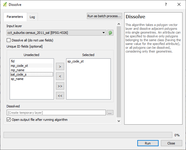
5. Merge by suburb (name) getting a multipolygon for repeated names

1. Census Small Area

For this data, ran the dissolve operation in QGIS on census_2011_sal on sal_code_s. There were severally named polygons, which is good for population related operations but not for the current geolocation exercise.

2. Official Planning Suburbs

This dataset had 792 records to start with, subsequently reduced to 776 features after removing slivers and ran single part to multipart to deal with polygon for non-contiguous areas.

3. Informal Areas

The informal settlement name was adopted for suburb at times the alias was used since this was referenced in the service requests.

4. Suburb Extras

At times neither the SAL nor the OFC Suburbs layer had data boundary data of an area. In such a case, OpenStreetMap was used as reference to define these and I created new areas where needed.

A Tables Grapple

All Together

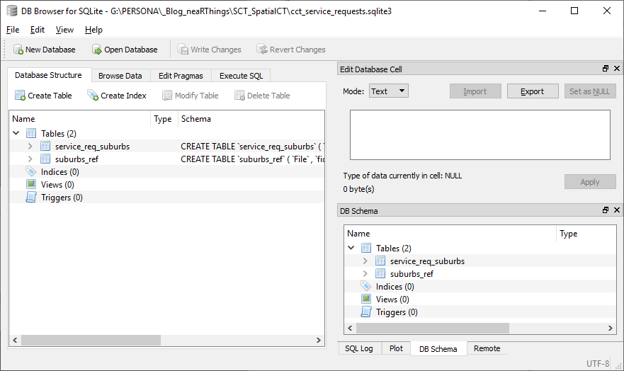
I exported only the suburb column of the service_request_2011 data from OR and imported the data into a sqlite database.

Similarly exported the attributes of the four suburb reference layers from QGIS as csv files, imported the quartet in OR and exported the compound to csv then importing into the database. This compound had 2139 records (non-unique as some names are common across the set).

There is a knowledge gap. I clearly see there is a better way to this process. This can all be done with some sql chops.

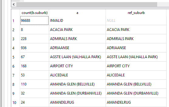
Next was to align the two tables, to which I resorted to

SELECT count(b.suburb), b.suburb AS a, c.suburb AS ref_suburb
 FROM service_req_suburbs AS b
 LEFT JOIN suburbs_ref AS c
 ON b.suburb = c.suburb
  GROUP BY a
  ORDER BY ref_suburb DESC;

The first run gave a gave a discrepancy of 486 viz records in service_req_suburbs layer and not the suburbs_ref.

I went back to OR, suburb by suburb, adjusting the suburb names, creating new place polygons if need be, until the two tables ‘aligned’.

Finally it came to this

Spatial Integrity

At this stage my spatial data is in a geopackage (essentially a sqlite database) and thus I can run spatial sql on it.

To check the validity of my spatial data (which i had not done until now, since my focus has been on attribute data), in QGIS, using the DB Manager i ran

SELECT suburb
FROM census_2011_sal
WHERE NOT ST_IsValid(geom);

for all the four layers. Turns out the geometry is valid as no feature(s) was returned.

What’s In A Place

This exercise has a local context and it makes sense when dealing with the geo data to think about projections. The most appropriate being South African CRS ZANGI:ZANGI:HBKNO19. I however postponed that for a later date and just went with EPSG 4326 instead. (* More on the HBKN019 can be gotten from here* and here ).

#PostScript

I moved my service_requests_2011 data from the sqlite database to the geopackage where the suburbs spatial data was.

The next step is to investigate closely the (X,Y) coordinate pair.